Advanced Excel Functions – DATE, VLOOKUP, and PMT Functions

Last updated on October 8th, 2023 at 02:40 pm

Advanced Excel functions will make your life easier on the job. From entering and changing information to doing calculations, graphing, and sorting data, Excel has all that you need. It is a great tool to make working with numbers easier and faster. Whether you are a business owner, office worker, or teacher, becoming a pro at using Excel will prove worthwhile.

If you are new to spreadsheets and have not seen them yet be sure to visit the introduction to spreadsheets and introduction to spreadsheet formulas. Additionally, visit what is a function for an introduction to functions and to learn some basic functions used in spreadsheets.

In this article, we will cover some advanced spreadsheet functions. Keek reading to learn:

• What is the Excel DATE function, and what is it used for;
• What the VLOKUP function is, and how to use it; and
• What is the PMT function, and how to use it.

There are many different brands of spreadsheet software. Be aware that this function may be different depending on the software. In this article, we are focusing on functions in Microsoft Excel.

The Excel DATE function

The date function is the spreadsheet function you use when we wish to enter dates in the form of day, month, and year. This function is able to format the data entered to match the number of days in a given month and the number of months in a given year.

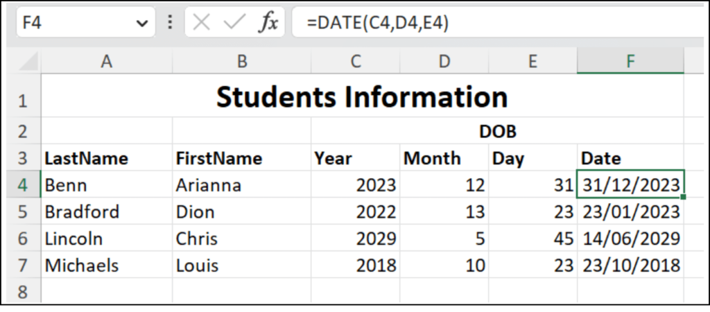
So in a situation where the user enters the day, month, and year information, the Date function can be used to combine these pieces of information, as shown in column F. See the format of the date function in F4.

If the user enters a number that is bigger than the expected number of days in the month, the spreadsheet adjusts the date. For instance, if you enter the 31st of February in a spreadsheet, the day would be automatically changed to the 3rd of March or the 2nd of March, depending on whether the year being entered is a leap year or not. See an example in F6 in the table above. In this instance, the month has 45 days which is impossible, so the number of days is carried over to the new month and is shown as day 14. You might notice that the original function had month 5, so the month is changed because of the number of days.

The VLOOKUP function – Advanced Excel functions

The VLOOKUP function is a very powerful tool you may use in Excel to search for data. In the instances where we have a large volume of data to sort through, the VLOOKUP function helps us to quickly search a table and find the particular piece of information we are looking for. For instance, we may search for a student’s name by entering their registration number in the VLOOKUP function. Let’s look at this with an example.

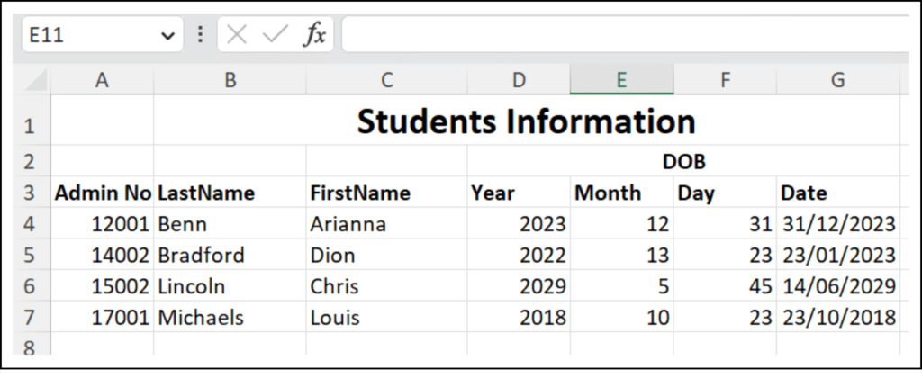
We are using the table below for this illustration.

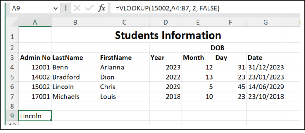
Let’s say we wish to find the name of the student whose registration number is 15002. Here is what we do. We create the VLOOKUP function, which has the 4 parameters which are explained below. For this explanation, we use: =VLOOKUP(15002, A4:B7, 2, FALSE).

1. The first parameter is the value we wish to find – 15002.
2. The second parameter is the area of the table that contains both the value we wish to find and the value we wish to display. In our case, we will use the first and second columns, so the range we use must contain the values of the first cell and the value of the last cell – A4:B7.
3. The third parameter is the place in the table where the data we wish to find is located. We use counting numbers to indicate the column. For instance, 1 indicates the first column, 2 is the second column, and so on. So because we are searching for a student whose admin number we know but whose name we need to find, we will enter 2 to indicate that we wish to print the name that matches that admission number. 2 indicates that the name is in the second column.
4. The last parameter is TRUE or FALSE. When we enter FALSE, we indicate that we are looking for an exact match for the admission. However, TRUE indicates that we are looking for an approximate match. It should be noted that using TRUE may cause some unexpected results.

See the actual function and results in the table below.

Now go ahead and give this a try for yourself.

The PMT function – Advanced Excel functions

The PMT function is a financial accounting function that helps you to calculate your monthly loan payments for a constant amount at a constant interest rate. It takes three to five parameters like this =PMT(rate, npr, Pv, [fv], [type] ), which are:

1. The rate is the interest you will pay on the loan expressed in percentage.
2. The second parameter npr is the number of monthly payments.
3. The pv refers to the principal, the actual amount of money borrowed.
4. The fourth parameter fv refers to the future value of your loan.
5. Type, which is the last parameter, uses values 1 or 0. These values refer to the time of the payments. If you set this value as 0 or omit it, this means that the payments are due at the end of the period. On the other hand,1 means your payments are due at the beginning of the period.

Note well the last two parameters are optional. The function will still work if you omit them. Below is a demonstration of this formula in use.

You may notice that the first parameter has the rate/12. This is because the rate given in the table is the annual interest rate. So we divide by 12 to get the monthly interest rate.

When you use the PMT function, the values will be negative. You may add a negative sign to make it positive. The answer represents your monthly loan amount.

If you found this article interesting, be sure to visit Excel conditional functions and analyzing data in Excel as well.

Before you go

We try our best to be as detailed and clear as possible in the information we provide. If you have any questions or comments, be sure to leave them in the comment section below.